Solar Disaggregation#
Author: Mohini Bariya
Date: May 20, 2021
This blog post uses the sunshine data to explore how much solar power is being generated on a network.
Solar Disaggregation#
Many regions, especially California, are seeing growing quantities of distributed solar generation, often in the form of PV panels installed on the rooftops of buildings and homes. These installations can inject power back into the electric grid through distribution networks, challenging the traditional uni-directional and centralized model of power systems. Even if a utility knows the size of PV installations on a particular distribution feeder, they have no real time visibility into the output of these PV units. Instead, all they can see is the net load, which is the difference between the full demand and PV output. This lack of visibility can result in a number of operational problems, including a reduced ability to predict rapid changes in net load arising from, say, a passing cloud that diminishes PV output.
Solar disaggregation techniques aim to solve this issue by estimating the full demand and PV output from measurements of net load. Disaggregation can occur at the scale of a home, an entire distribution feeder, or a full interconnection.
We will try to perform solar disaggregation for the PV feeder in the sunshine dataset. As a reminder, Fig. 1 shows the configuration of PMUs in this dataset.
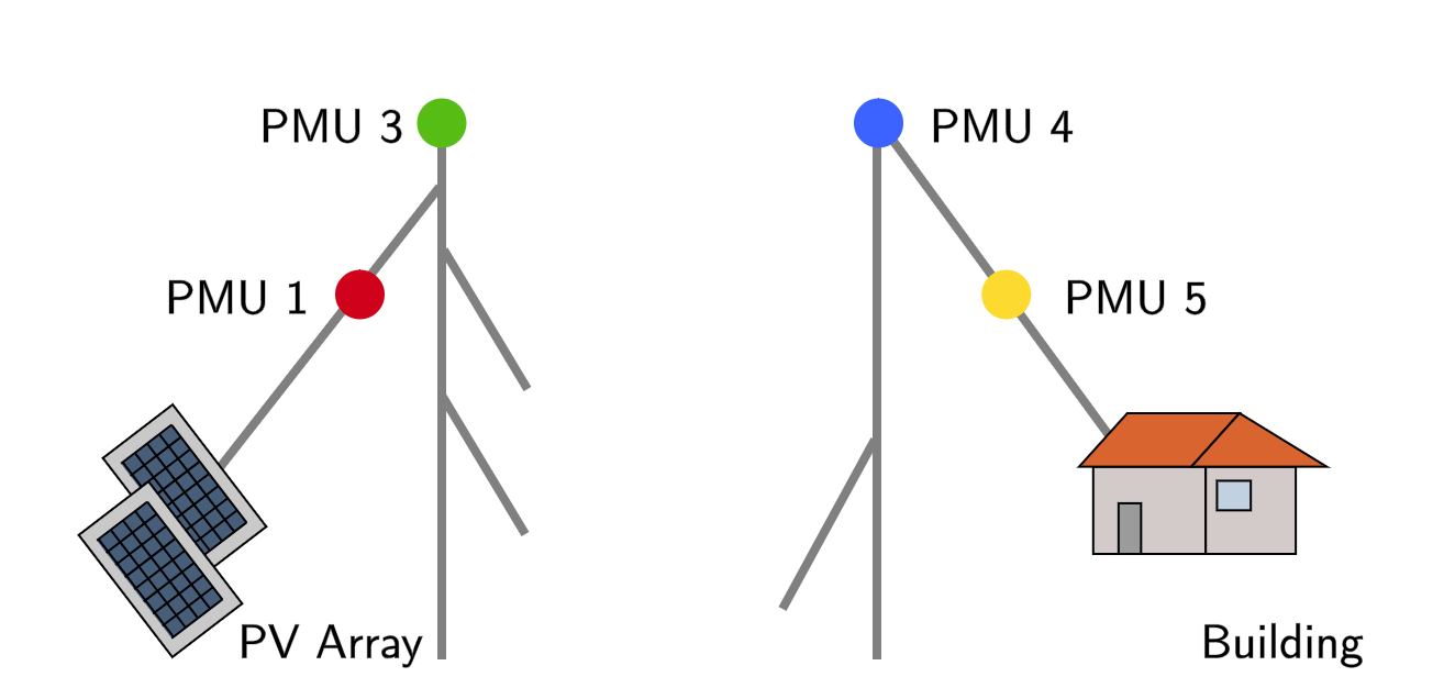 Figure 1: PMUs 1, 3, 4, and 5 in the sunshine dataset. PMUs 3 & 4 are at the heads of two separate feeders. PMU 1 measures the interconnection of a PV array below PMU 3. PMU 5 measures the interconnection of a building below PMU 4.
We will use only measurements from PMU 3 at the feeder head. In the case of sunshine, we actually have a direct measurement of the PV output from PMU 1, but the intended application of this technique is to feeders with no direct measurements of PV output. Our disaggregation approach is a simplification of the technique in [1], and relies on the power factor, which was introduced on a previous blog post. When applied to an arbitrary feeder, the technique will not reveal anything about the location and number of PV installations. Instead, given measurements of net load, it will reveal the aggregate PV output and the aggregate demand over the entire feeder.
The crucial assumption of the algorithm is that the aggregate power factor of the feeder sans the PV installation is constant. When the PV installation outputs real power, this will change the net real power demand and therefore the aggregate power factor as measured at PMU 3 (visualized in Fig. 2).
 Figure 2: Visualizing how PV output changes the complex power angle (and equivalently the power factor) of the net load measured at PMU 3 from $\theta$ to $\theta’$. We assume that $\theta$ is constant for the purposes of disaggregation.
We will express $P_1$, the power output of the PV, as a factor of $P$, the real power demand of the feeder:
$$ P_1 = fP $$
The net real power load measured at PMU 3 is $P - P_1 = (1-f)P$. Our disaggregation algorithm will estimate the factor $f$. Given $\theta$ and a measurement of $\theta’$ (the power angles with and without PV output, which could be substituted with power factors $pf$ and $pf’$) we can solve for $f$ as follows.
First, we convert from power factor to the ratio between real and reactive power, denoted $\tau$:
$$ \begin{aligned} \tau \triangleq \tan(\theta) = \tan(\cos^{-1}(pf)) = \frac{Q}{P}\ \tau’ = \tan(\theta’) = \tan(\cos^{-1}(pf’)) = \frac{Q}{(1-f)P} \ \therefore \tau’ = \frac{\tau P}{(1-f)P} = \frac{\tau}{1-f} \end{aligned} $$ Then we solve for $f$: $$ \begin{aligned} \implies f = 1 - \frac{\tau}{\tau’} \end{aligned} $$
To obtain $\theta$ or $pf$—which correspond to the aggregate feeder demand and are assumed constant—we can look at the power flow into the feeder during nighttime hours, when PV output is zero. Using this constant value, we can then determine $f$ at various time points during daytime hours from measurements of the power factor or $\theta’$ at those times.
We apply this approach to data from PMU 3. We set $pf$ to a constant value equal to the average of the measured power factor at night over several days. Then, given the measured power factor at some time in the day, we use the equations above to compute $f$. The results are plotted in Fig. 3, visualized just as power factors were visualized earlier.
 Figure 3: Estimates of the disaggregation factor $f$ at each hour of the day on each day of the week over several weeks.
A value of $f = 1$ implies that the power output of the PV exactly matches the real power demand on the feeder. This will result in zero real power flow from the bulk grid to the feeder through PMU 3. When $f < 1$, the PV output is insufficient to meet feeder demand, and the shortfall will be drawn from the bulk grid. When $f > 1$, there is a surplus of PV generation, and the excess will flow from the feeder into the main grid, resulting in reverse power flow.
We see that during the peak PV output hours, $f$ often exceeds $1$, resulting in reverse power flow. There is a distinctive weekly trend, with $f$ being significantly larger on weekends, not because of a major change in PV output but presumably due to a marked drop in demand.
References#
Kara, E. C., Roberts, C. M., Tabone, M., Alvarez, L., Callaway, D. S., & Stewart, E. M. (2016). Towards real-time estimation of solar generation from micro-synchrophasor measurements. arXiv preprint arXiv:1607.02919.