9 - Visualizing Aggregates#
This tutorial brings together concepts from previous posts around data visualization, statpoints, and windows queries. The visualizations provided below offer a powerful tool for visualizing arbitrarily long time series of data, while also highlighting specific regions in the data that may be of interest.
We also provide two helper functions which may be useful for other user-developed code. The first (points_to_dataframe) takes a list of StatPoint objects returned from a btrdb windows queries and converts it into a Pandas dataframe, where the columns are StatPoint attributes (i.e., min, max, mean, standard deviation and count). The second helper function (plot_aggregates) uses this Pandas dataframe to generate a plot showing the range and distribution of values over time.
[1]:
import btrdb
import pandas as pd
import numpy as np

import time


from datetime import datetime, timedelta

from matplotlib import pyplot as plt
from btrdb.utils import timez

db = btrdb.connect()
Select data#
[2]:
streams = db.streams_in_collection('sunshine/PMU1', tags={'unit': 'volts'})

pd.DataFrame([[s.name, s.unit, s.collection] for s in streams],
            columns=['name','unit','collection'])
[2]:
| name | unit | collection | |
|---|---|---|---|
| 0 | L3MAG | volts | sunshine/PMU1 |
| 1 | L1MAG | volts | sunshine/PMU1 |
| 2 | L2MAG | volts | sunshine/PMU1 |
Determine time interval#
Below, we use stream.earliest() and stream.latest() to determine the time interval spanned by the data.
[3]:
stream = db.stream_from_uuid(streams[1].uuid)

def get_time(stream, func):
    return timez.ns_to_datetime(getattr(stream, func)()[0].time)

print('start:', get_time(streams[0], 'earliest'))
print('end:', get_time(streams[0], 'latest'))
print(str(get_time(streams[0], 'latest') - get_time(streams[0], 'earliest')))
start: 2015-10-01 16:08:24.008333+00:00
end: 2017-04-15 01:41:35.999999+00:00
561 days, 9:33:11.991666
See it in the plotter: https://plot.ni4ai.org/permalink/VKne4LTTl
Choose time interval#
Here, we select a time interval of one year.
[4]:
start_time = datetime(2016,4,1)
end_time = datetime(2017,4,1)

start_ns = timez.datetime_to_ns(start_time)
end_ns = timez.datetime_to_ns(end_time)
https://plot.ni4ai.org/permalink/2KN5iCXw5
[5]:
window = timez.ns_delta(days=30)
pw = int(np.log2(window))

points, _ = zip(*stream.aligned_windows(start_ns, end_ns, pointwidth=pw))
points
[5]:
(StatPoint(1459166279268040704, 6825.37109375, 7157.580867829119, 7301.88525390625, 269591739, 36.51418677591111),
 StatPoint(1461418079081725952, 6580.9541015625, 7161.23304578515, 7300.8623046875, 269692154, 35.61453444076186),
 StatPoint(1463669878895411200, 6796.833984375, 7160.458736401789, 7286.55126953125, 147383982, 34.1646855496053),
 StatPoint(1465921678709096448, 6964.91455078125, 7159.378036144785, 7325.37158203125, 206497053, 40.14920297145494),
 StatPoint(1468173478522781696, 5558.57421875, 7167.452925690963, 7294.76318359375, 269810992, 39.238088874956624),
 StatPoint(1470425278336466944, 5780.056640625, 7161.174368865373, 7307.212890625, 268549058, 41.321696619794494),
 StatPoint(1472677078150152192, 6392.52099609375, 7161.894405845441, 7318.228515625, 268988146, 39.96141042153979),
 StatPoint(1474928877963837440, 5955.3212890625, 7158.670968887105, 7300.72509765625, 255962541, 39.97700500308349),
 StatPoint(1477180677777522688, 5097.31298828125, 7156.974233908252, 7283.45361328125, 268787149, 36.33054088798969),
 StatPoint(1479432477591207936, 6591.23486328125, 7158.855179375172, 7281.74755859375, 270215978, 33.48565115468457),
 StatPoint(1481684277404893184, 6501.1142578125, 7162.591062269605, 7282.77734375, 270216211, 34.53212742881303),
 StatPoint(1483936077218578432, 6076.43017578125, 7162.1296525714415, 7262.462890625, 270089894, 35.17972671790351),
 StatPoint(1486187877032263680, 6127.64404296875, 7153.473267831473, 7292.42724609375, 234816262, 37.10013475124324),
 StatPoint(1488439676845948928, 5907.42041015625, 7160.925875368738, 7297.984375, 270196174, 34.90643606628646))
Convert to pandas dataframe#
[6]:
def points_to_dataframe(points,
                        aggregates=['time','min','max','mean','stddev','count'],
                        use_datetime_index=True):
    df = pd.DataFrame([[getattr(p, agg) for agg in aggregates] for p in points],
                         columns=aggregates)
    if use_datetime_index:
        df['datetime'] = [timez.ns_to_datetime(t) for t in df.time]
        df = df.set_index('datetime')
    return df

df = points_to_dataframe(points)
df
[6]:
| time | min | max | mean | stddev | count | |
|---|---|---|---|---|---|---|
| datetime | ||||||
| 2016-03-28 11:57:59.268041+00:00 | 1459166279268040704 | 6825.371094 | 7301.885254 | 7157.580868 | 36.514187 | 269591739 |
| 2016-04-23 13:27:59.081726+00:00 | 1461418079081725952 | 6580.954102 | 7300.862305 | 7161.233046 | 35.614534 | 269692154 |
| 2016-05-19 14:57:58.895411+00:00 | 1463669878895411200 | 6796.833984 | 7286.551270 | 7160.458736 | 34.164686 | 147383982 |
| 2016-06-14 16:27:58.709096+00:00 | 1465921678709096448 | 6964.914551 | 7325.371582 | 7159.378036 | 40.149203 | 206497053 |
| 2016-07-10 17:57:58.522782+00:00 | 1468173478522781696 | 5558.574219 | 7294.763184 | 7167.452926 | 39.238089 | 269810992 |
| 2016-08-05 19:27:58.336467+00:00 | 1470425278336466944 | 5780.056641 | 7307.212891 | 7161.174369 | 41.321697 | 268549058 |
| 2016-08-31 20:57:58.150152+00:00 | 1472677078150152192 | 6392.520996 | 7318.228516 | 7161.894406 | 39.961410 | 268988146 |
| 2016-09-26 22:27:57.963837+00:00 | 1474928877963837440 | 5955.321289 | 7300.725098 | 7158.670969 | 39.977005 | 255962541 |
| 2016-10-22 23:57:57.777523+00:00 | 1477180677777522688 | 5097.312988 | 7283.453613 | 7156.974234 | 36.330541 | 268787149 |
| 2016-11-18 01:27:57.591208+00:00 | 1479432477591207936 | 6591.234863 | 7281.747559 | 7158.855179 | 33.485651 | 270215978 |
| 2016-12-14 02:57:57.404893+00:00 | 1481684277404893184 | 6501.114258 | 7282.777344 | 7162.591062 | 34.532127 | 270216211 |
| 2017-01-09 04:27:57.218578+00:00 | 1483936077218578432 | 6076.430176 | 7262.462891 | 7162.129653 | 35.179727 | 270089894 |
| 2017-02-04 05:57:57.032264+00:00 | 1486187877032263680 | 6127.644043 | 7292.427246 | 7153.473268 | 37.100135 | 234816262 |
| 2017-03-02 07:27:56.845949+00:00 | 1488439676845948928 | 5907.420410 | 7297.984375 | 7160.925875 | 34.906436 | 270196174 |
Define data viz helper function#
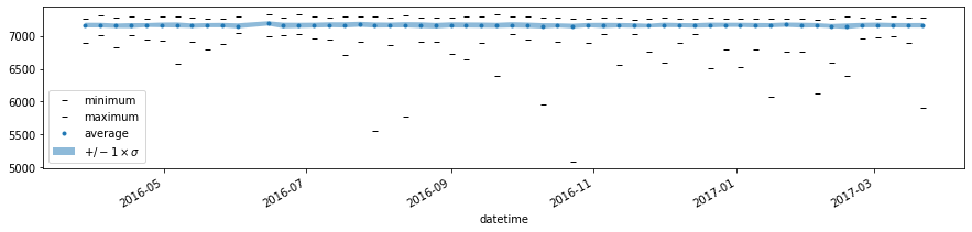
[7]:
def plot_aggregates(df, vlines=[], hlines=[]):
    fig, ax = plt.subplots(figsize=(15,3))
    df['min'].plot(ax=ax, ls=' ', marker='_', color='black', markersize=5, label='minimum')
    df['max'].plot(ax=ax, ls=' ', marker='_', color='black', markersize=5, label='maximum')
    df['mean'].plot(ax=ax, label='average', ls=' ', marker='.')
    ax.fill_between(df.index, df['mean']-df['stddev'], df['mean'] + df['stddev'], alpha=0.5, label=r'$+/- 1\times\sigma$')
    plt.legend()

    ax.vlines(vlines, *ax.get_ylim(), color='0.5', alpha=0.5, zorder=10, lw=3, label='events')
    ax.hlines(hlines, *ax.get_xlim(), color='0.5', zorder=10, lw=1, ls='--', label='threshold')
    return fig

plot_aggregates(df)
plt.show()

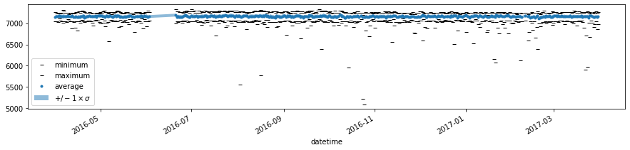
Visualize aggregates at different time-resolutions#
Weekly#
[8]:
window = timez.ns_delta(days=7)
pw = int(np.log2(window))

points, _ = zip(*stream.aligned_windows(start_ns, end_ns, pointwidth=pw))
df = points_to_dataframe(points)
fig = plot_aggregates(df)
Daily#
[9]:
window = timez.ns_delta(days=1)
pw = int(np.log2(window))

points, _ = zip(*stream.aligned_windows(start_ns, end_ns, pointwidth=pw))
df = points_to_dataframe(points)
fig = plot_aggregates(df)
[ ]: