0 - PredictiveGrid in Python

A Quick Start Notebook

This notebook is a quick start to working with data using PredictiveGrid’s Python API. It illustrates the basic, key functionality of the API to give you a running start working with data in the platform.

The very first step is to import all the required packages. Below is a list of basic imports that you can copy and paste into your own notebooks to get going. The external python libraries (matplotlib, numpy, etc.) have wonderful, extensive documentation that you should look up if you want to explore all their functionalities or just unstick yourself. The %matplotlib inline command ensures that plots will be rendered in the notebook itself, rather than in a pop-up window.

# PredictiveGrid imports
import btrdb # Platform Python bindings
from btrdb.utils import timez # helpful sub-package for handling time
from btrdb.stream import StreamSet # subpackage with light wrapper for working with multiple streams

# External Python libraries
import numpy as np # scientific computing package
import matplotlib.pyplot as plt # plotting package
import pandas as pd # data analysis library
from tabulate import tabulate # creating & printing neat tables
from datetime import datetime, timedelta # for working with time

%matplotlib inline

Next, we must connect to the database. The connect function optionally accepts endpoint and apikey string arguments, which can be passed like:

btrdb.connect(endpoint_string, apikey=key_string)

When running a notebook on JupyterHub, these do not need to be passed.

conn = btrdb.connect()
conn.info()

{'majorVersion': 5, 'build': '5.12.5', 'proxy': {'proxyEndpoints': []}}

Find Collections

The streams in the database are organized into collections, which can be thought of as heirarchical paths such as CALIFORNIA/SanFrancisco/91405/Sensor1 but are internally just strings. A single collection, defined by a path-like name, can contain any number of individual streams. It is best to name collections and organize streams into them in some logically consistent and descriptive way to facilitate searching (think about creating a file heirarchy to organize data files and mirror this in the collection name).

Let us query all and print out some of the collections in this cluster. We will print out the individual collection names to reflect the implicit heirarchical data organization they encode.

collections = conn.list_collections()
print('Found', len(collections), 'collections')

collections.sort()

# We limit the number of collections so we don't print too many
for i, c in enumerate(collections[0:3]):
    levels = c.split('/')
    for j, l in enumerate(levels):
        if i == 0:
            pass
        elif l in collections[i-1]:
            continue
        print(j*' ','->', l)

Found 486 collections
 -> Health
  -> EKG
   -> patient001
 -> POW
  -> EPFL
  -> GridSweep

We can also limit the search to collections with a certain prefix (you may want to change the prefix below to obtain interesting results on your particular allocation).

prefix = 'sunshine/PMU1'
collections = conn.list_collections(prefix)

print('Found', len(collections), 'collections')
print(collections)

Found 1 collections
['sunshine/PMU1']

Find Streams

Now that we have a collection, the next step is to find individual streams (though we could have done this directly, if we know what we want). As you may recall, each stream represents a single time series within the database, which contains the atomic, (time, value) pairs, and has some associated metadata.

To get the streams, we will use the streams_in_collection method. This takes an optional collection prefix argument. If we pass in no argument, we will get all streams in the database. Let us work with the collection we found previously. Note that the method returns an iterator, which we convert to a list below.

collection = collections[0]
streams = list(conn.streams_in_collection(collection))
print('Found', len(streams), 'streams in collection', collection)

Found 13 streams in collection sunshine/PMU1

Recall that streams have metadata, which can help us understand what the stream is. The convenience function below will obtain and pretilly print a set of streams and their metadata.

def describe_streams(streams):
    table = [["Collection", "Name", "Units", "Version", "UUID"]]
    for stream in streams:
        # Get all the tags for this stream.
        tags = stream.tags()
        table.append([
            stream.collection, stream.name, tags["unit"], stream.version(), stream.uuid
        ])
    return tabulate(table, headers="firstrow")

print(describe_streams(streams))

Collection     Name    Units      Version  UUID
-------------  ------  -------  ---------  ------------------------------------
sunshine/PMU1  LSTATE  mask        243640  6ffb2e7e-273c-4963-9143-b416923980b0
sunshine/PMU1  C1ANG   deg         240607  d625793b-721f-46e2-8b8c-18f882366eeb
sunshine/PMU1  C3MAG   amps        240481  fb61e4d1-3e17-48ee-bdf3-43c54b03d7c8
sunshine/PMU1  C2MAG   amps        240718  d765f128-4c00-4226-bacf-0de8ebb090b5
sunshine/PMU1  C1MAG   amps        240380  1187af71-2d54-49d4-9027-bae5d23c4bda
sunshine/PMU1  C3ANG   deg         240781  0be8a8f4-3b45-4fe3-b77c-1cbdadb92039
sunshine/PMU1  L3ANG   deg         240862  e4efd9f6-9932-49b6-9799-90815507aed0
sunshine/PMU1  L2ANG   deg         240662  886203ca-d3e8-4fca-90cc-c88dfd0283d4
sunshine/PMU1  L3MAG   volts       229263  b2936212-253e-488a-87f6-a9927042031f
sunshine/PMU1  L1ANG   deg         229265  51840b07-297a-42e5-a73a-290c0a47bddb
sunshine/PMU1  C2ANG   deg         229263  97de3802-d38d-403c-96af-d23b874b5e95
sunshine/PMU1  L1MAG   volts       229266  35bdb8dc-bf18-4523-85ca-8ebe384bd9b5
sunshine/PMU1  L2MAG   volts       229264  d4cfa9a6-e11a-4370-9eda-16e80773ce8c

We can also search for streams in terms of their metadata tags, by passing an optional tag arguement to the same streams_in_collection method. Let us get all the streams with units of volts.

streams = conn.streams_in_collection(collection, tags={"unit": "volts"})
print(describe_streams(streams))

Collection     Name    Units      Version  UUID
-------------  ------  -------  ---------  ------------------------------------
sunshine/PMU1  L3MAG   volts       229263  b2936212-253e-488a-87f6-a9927042031f
sunshine/PMU1  L1MAG   volts       229266  35bdb8dc-bf18-4523-85ca-8ebe384bd9b5
sunshine/PMU1  L2MAG   volts       229264  d4cfa9a6-e11a-4370-9eda-16e80773ce8c

The API also supports SQL queries to find streams and metadata, which you can learn more about in this notebook.

Work with a stream

Let us work with the first stream in the above list of streams. We will look at its metadata and learn how to query time series data from the stream.

stream = streams[0]
print(stream)

<Stream collection=sunshine/PMU1 name=L3MAG>

Let’s checkout the stream’s metadata. Note that stream.tags() returns a dictionary of tags, while stream.annotations returns a tuple, where the first element is the annotation version and the second is the dictionary of annotations.

print('COLLECTION:', stream.collection)

print('\nTAGS:\n', stream.tags().keys())
print('\nANNOTATIONS:\n', stream.annotations()[0].keys(),)

COLLECTION: sunshine/PMU1

TAGS:
 dict_keys(['unit', 'ingress', 'distiller', 'name'])

ANNOTATIONS:
 dict_keys(['location', 'impedance'])

Data Types from Time Series Queries

Before we move on, let’s refresh some concepts on BTrDB data types.

There are two data types (represented by Python objects) that we may obtain when querying time series data from a stream. These are:

1. RawPoints — RawPoints represent the atomic data type in a time series: a paired timestamp and value that is the raw data of the series. Recall that these are stored at the absolute bottom of the BTrDB tree.

2. StatPoints — These are stored in the internal nodes of the BTrDB tree and contain precomputed statistical aggregates of the raw data that lies beneath them.

Querying RawPoints will be slower than querying StatPoints. Between StatPoints, it is faster to query those that reside higher up in the tree, corresponding to longer durations of raw data and correspondingly larger numbers of RawPoints.

Data Time Range

There are a couple useful methods for understanding the time range covered by a stream. We can do this by getting the earliest and latest RawPoints in the stream, as shown below.

A few things: queries for time series Points always return the Point(s) requested along with a *version number*. For most introductory users, the version is not useful, though you can read more about it in our docs. Below, we discard the version and just work with the returned RawPoint.

Time stamps in BTrDB are integers which represent nanoseconds since the Unix epoch (January 1, 1970). These can be easily converted to more readable time stamps using utility functions in the timez package (read the docs here).

# Get the earliest & latest RawPoints in the stream
earliest, version = stream.earliest()
latest, version = stream.latest()

# Get the time from the RawPoints
earliest_time = earliest.time
latest_time = latest.time

print('Stream starts at: ', timez.ns_to_datetime(earliest_time))
print('Stream ends at: ', timez.ns_to_datetime(latest_time))

Stream starts at:  2015-10-01 16:08:24.008333+00:00
Stream ends at:  2017-04-15 01:41:35.999999+00:00

Querying Data

There are three different methods to query data from a stream. These are documented & described below (in order of increasing query speed). 1. stream.values(start, end): This call will return all RawPoints in the stream between the start and end time. 2. stream.windows(start, end, width, depth=0): This call will return StatPoints spanning (and summarizing) windows of length width between the start and end times. The widtharguement is an integer specifying the window length in nanoseconds. The optional integer depth parameter trades off the precision of the window width for efficiency. It is specified as a power of \(2\) in nanoseconds (so depth=30 would make the windows accurate to roughly one second). 3. stream.aligned_windows(start, end, pointwidth): Like stream.windows, this call will return StatPoints corresponding to windows of a given width between the start and end times. However, this time, the width is specified as an integer power of \(2\) in nanoseconds in the pointwidth argument.

To reiterate, values returns RawPoints, while windows and aligned_windows return StatPoints.

All these queries return a list of tuples, where each tuples contains a Point (RawPoint or StatPoint) and a version number. Further, as mentioned, the time stamps in the Points are in the inconvenient nanoseconds since the Unix epoch format.

Overall, we need a function to convert this returned data into a more conducive format. We choose to convert the RawPoints to a pandas Series, and the StatPoints to a pandas DataFrame, which are easy to work with. The functions to do this are defined below (these can be easily modified to produce a numpy.array if desired).

def rawpoints_to_series(rawpts_response):
    times, values = [], []
    for rawpoint, version in rawpts_response:
        times.append(timez.ns_to_datetime(rawpoint.time))
        values.append(rawpoint.value)
    return pd.Series(index=times, data=values)

def statpoints_to_dataframe(statpoints):
    attributes = ['min','mean','max','stddev','count','time',]

    df = pd.DataFrame([[getattr(p, attr) for attr in attributes] for p, version in statpoints],
                     columns=attributes)

    df['datetime'] = [timez.ns_to_datetime(t) for t in df['time']]
    return df.set_index('datetime')

stream.values

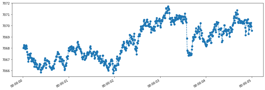
Let us choose a start and end time for a values query. CAUTION: Most streams contain very high frequency data, so don’t use too long a duration when querying raw data.

start = datetime(2015, 10, 10)
end = start + timedelta(seconds=5)

# Query the data
rawpts_response = stream.values(start, end)
# Convert it to a pandas Series
data = rawpoints_to_series(rawpts_response)

It is very easy to plot the data in a pandas series. Just call plot()! Here we pass a few aesthetic arguments to the call.

data.plot(linestyle='--', marker='o', figsize=(15, 5));

stream.windows

Let us choose a longer time range and a window length for a windows query, which will return StatPoints. Remeber that the window width must be specified as an integer number of nanoseconds.

start = datetime(2015, 10, 10)
end = start + timedelta(hours=24)
width = timedelta(minutes=1)
width_ns = int(1e9*width.seconds)

# Query the data
statpts_response = stream.windows(start, end, width_ns)
# Convert it to a pandas Series
data = statpoints_to_dataframe(statpts_response)

You can think of a pandas DataFrame as an excel file. In this case, the rows are timestamps (coressponding to the windows) and the columns contain the different aggregates.

We can visualize the dataframe structure and entries with the head() call.

data.head()

	min	mean	max	stddev	count	time
datetime
2015-10-10 00:00:00+00:00	7059.082520	7070.945893	7077.476562	2.470590	7200	1444435200000000000
2015-10-10 00:01:00+00:00	7043.672852	7058.894961	7069.110840	3.957179	7200	1444435260000000000
2015-10-10 00:02:00+00:00	7034.760254	7053.560129	7060.030762	4.170064	7200	1444435320000000000
2015-10-10 00:03:00+00:00	7041.854004	7053.804716	7058.428223	2.277033	7200	1444435380000000000
2015-10-10 00:04:00+00:00	7040.025879	7055.781075	7059.692383	1.901117	7200	1444435440000000000

Let us plot the resulting data. We can call .plot() on the DataFrame, as we did earlier, but instead, we will manually plot only some of the columns, for easier and greater control of the visualization.

plt.figure(figsize=(15, 5))
# Plot the mean of the windows
plt.plot(data.index, data['mean'], linewidth=2, color='red', linestyle='--', marker='o')
# Show the range of the minimum and maximum over the windows
plt.fill_between(data.index, data['min'], data['max'], color='lightgrey')

<matplotlib.collections.PolyCollection at 0x7f981c0be080>

stream.aligned_windows

Let us use the same start and end times in an aligned_windows query. Now, however, the window width must be an integer power of \(2\) nanoseconds, termed a pointwidth. The following function will convert an arbitrary timedelta into the nearest pointwidth, and return the error (in seconds) between the input and returned widths.

def to_nearest_pointwidth(dt):
    dt_ns = 1e9*dt.seconds
    prevpw = int(np.floor(np.log2(dt_ns)))
    nextpw = int(np.ceil(np.log2(dt_ns)))

    preverr = (dt_ns-(2**prevpw)) / 1e9
    nexterr = ((2**nextpw)-dt_ns) / 1e9

    if preverr <= nexterr:
        return prevpw, preverr
    else:
        return nextpw, nexterr

print(to_nearest_pointwidth(timedelta(seconds=1)))

(30, 0.073741824)

start = datetime(2015, 10, 10)
end = start + timedelta(hours=24)
width = timedelta(minutes=1)
pw, err = to_nearest_pointwidth(width)

print('pointwidth', pw, 'with error', err, 'seconds')

pointwidth 36 with error 8.719476736 seconds

# Query the data
statpts_response = stream.aligned_windows(start, end, pw)
# Convert it to a pandas Series
data = statpoints_to_dataframe(statpts_response)

plt.figure(figsize=(15, 5))
# Plot the mean of the windows
plt.plot(data.index, data['mean'], linewidth=2, color='red', linestyle='--', marker='o')
# Show the range of the minimum and maximum over the windows
plt.fill_between(data.index, data['min'], data['max'], color='lightgrey')

<matplotlib.collections.PolyCollection at 0x7f981c144f60>

What if we specify a longer window?

start = datetime(2015, 10, 10)
end = start + timedelta(hours=24)
width = timedelta(minutes=10)
pw, err = to_nearest_pointwidth(width)

print('pointwidth', pw, 'with error', err, 'seconds')

# Query the data
statpts_response = stream.aligned_windows(start, end, pw)
# Convert it to a pandas Series
data = statpoints_to_dataframe(statpts_response)

plt.figure(figsize=(15, 5))
# Plot the mean of the windows
plt.plot(data.index, data['mean'], linewidth=2, color='red', linestyle='--', marker='o')
# Show the range of the minimum and maximum over the windows
plt.fill_between(data.index, data['min'], data['max'], color='lightgrey');

pointwidth 39 with error 50.244186112 seconds

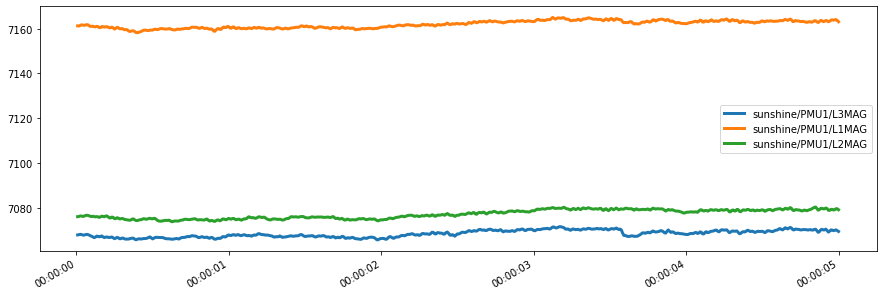
Work with multiple streams using streamsets

We often want to query data from a bunch of streams. Of course, we could do this manually by iterating through the individual streams and using the methods described. However, we also have the option of using a `StreamSet <https://btrdb.readthedocs.io/en/latest/working/streamsets.html>`__, which is a light wrapper around a list of streams.

The following cells show a few examples for working with StreamSets. For more, see this notebook. Notice that when querying StreamSets, version numbers are no longer returned, as they were for queries on single streams.

To begin, we use the same collection as before, and get a list of streams, which we then convert to a StreamSet.

streams = conn.streams_in_collection(collection, tags={"unit": "volts"})
streamset = StreamSet(streams)

We can now do some queries on all streams at once. For example…

earliests = streamset.earliest() # Returns a list of RawPoints, one for each stream
latests = streamset.latest() # Returns a list of RawPoints, one for each stream

for i in range(len(streamset)):
    # Get the times for this stream
    earliest_time = earliests[i].time
    latest_time = latests[i].time
    print('Stream', streamset[i].name)
    print('starts at: ', timez.ns_to_datetime(earliest_time))
    print('ends at: ', timez.ns_to_datetime(latest_time))
    print('--------------------')

Stream L3MAG
starts at:  2015-10-01 16:08:24.008333+00:00
ends at:  2017-04-15 01:41:35.999999+00:00
--------------------
Stream L1MAG
starts at:  2015-10-01 16:08:24.008333+00:00
ends at:  2017-04-15 01:37:11.333333+00:00
--------------------
Stream L2MAG
starts at:  2015-10-01 16:08:24.008333+00:00
ends at:  2017-04-15 01:41:35.999999+00:00
--------------------

Let us make a values (ie raw data) query on this StreamSet. Notice the difference in the query form: we use a function chaining approach to first set the start and end times. Then, the values are requested.

start = datetime(2015, 10, 10)
end = start + timedelta(seconds=5)
data = streamset.filter(start, end).values()

The result data, is a list of lists, each containing the RawPoints for one of the streams in the StreamSet.

To make the data more workable, we can instead query the result as a pandas DataFrame, as shown below:

data = streamset.filter(start, end).to_dataframe()

data.head()

	sunshine/PMU1/L3MAG	sunshine/PMU1/L1MAG	sunshine/PMU1/L2MAG
time
1444435200008333000	7068.010742	7161.215332	7076.146484
1444435200016666000	7068.098633	7161.130371	7076.227539
1444435200024999000	7068.275879	7161.411133	7076.442383
1444435200033333000	7068.182617	7161.659668	7076.458984
1444435200041666000	7067.982422	7161.583008	7076.268066

The timestamps still need to be converted, which we do below:

def to_human_time(time_ns):
    time_human = []
    for time in time_ns:
        time_human.append(timez.ns_to_datetime(time))
    return time_human

data.index = to_human_time(data.index)

data.head()

	sunshine/PMU1/L3MAG	sunshine/PMU1/L1MAG	sunshine/PMU1/L2MAG
2015-10-10 00:00:00.008333+00:00	7068.010742	7161.215332	7076.146484
2015-10-10 00:00:00.016666+00:00	7068.098633	7161.130371	7076.227539
2015-10-10 00:00:00.024999+00:00	7068.275879	7161.411133	7076.442383
2015-10-10 00:00:00.033333+00:00	7068.182617	7161.659668	7076.458984
2015-10-10 00:00:00.041666+00:00	7067.982422	7161.583008	7076.268066

And we can plot!

data.plot(figsize=(15, 5), linewidth=3)

<AxesSubplot:>

And that is it! You’ve had a basic introduction to working with PredictiveGrid in Python. You are ready to start working with your data and conducting some interesting analyses.

As you go, you will want to learn about and use more advanced platform capabilities. Make sure to look at the notebooks here containing both tutorials and analytics demos. You can also read the blog, which shares user stories, capabilities, etc. Also, read the docs!

THE END